Sweeping variables and inspecting fields

To optimize micromagnet designs it is possible to sweep one or two variables in the simulation. For each point in this sweep properties at the locations of the pre-defined qubit can be inspected. As an example, the following micromagnet design will be used :

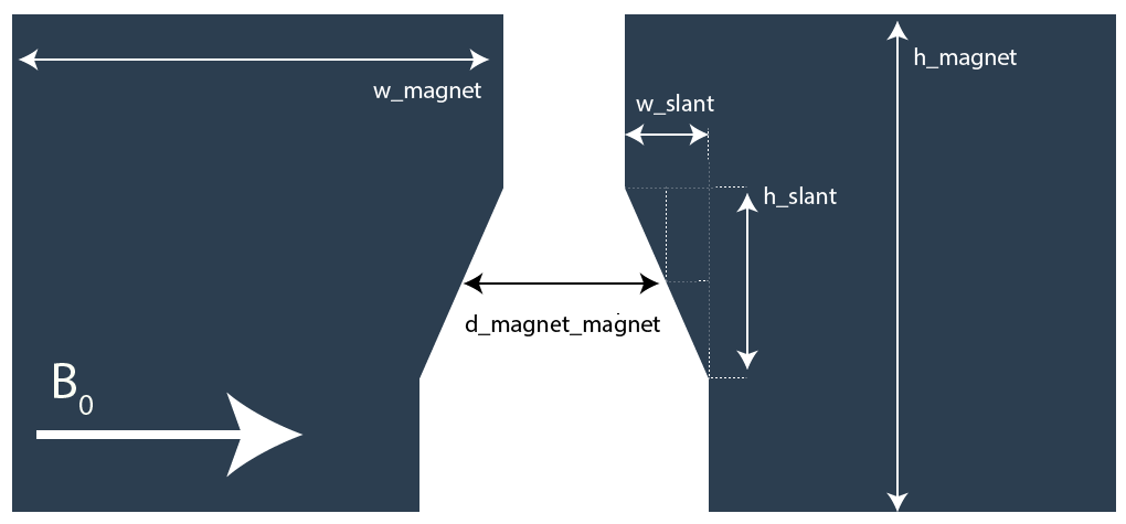
Let’s start by making a function that generaties this design:

from micromagnet_simulator.magnet_creator import umag_creator

def example_MM_design(d_magnet_magnet, h_slant, w_slant, h_2deg=70, h_magnet=200):
        w_magnet = 5000
        h_magnet = 2000


        umag = umag_creator()
        umag.set_magnetisation(1,0,0)

        umag.add_electron_position(0, -200, -30)
        umag.add_electron_position(0, -120, -30)
        umag.add_electron_position(0,  -40, -30)
        umag.add_electron_position(0,   40, -30)
        umag.add_electron_position(0,  120, -30)
        umag.add_electron_position(0,  200, -30)


        # the big slabs
        umag.add_cube(-w_magnet/2-d_magnet_magnet/2-w_slant/2, 0, h_2deg+h_magnet/2,
                w_magnet,h_magnet,h_magnet)
        umag.add_cube( w_magnet/2+d_magnet_magnet/2+w_slant/2, 0, h_2deg+h_magnet/2,
                w_magnet,h_magnet,h_magnet)

        # the small pieces above the rectangle
        umag.add_cube(-d_magnet_magnet/2, h_magnet/4+h_slant/4, h_2deg+h_magnet/2,
                w_slant,h_magnet/2-h_slant/2,h_magnet)
        umag.add_cube( d_magnet_magnet/2, h_magnet/4+h_slant/4, h_2deg+h_magnet/2,
                w_slant,h_magnet/2-h_slant/2,h_magnet)

        # the rectangular pieces.
        p_2 = (-d_magnet_magnet/2-w_slant/2, -h_slant/2, h_2deg+h_magnet/2)
        p_1 = (-d_magnet_magnet/2-w_slant/2,  h_slant/2, h_2deg+h_magnet/2)
        p_3 = (-d_magnet_magnet/2+w_slant/2,  h_slant/2, h_2deg+h_magnet/2)
        umag.add_triangle(*p_1, *p_2, *p_3, 'z',200, n_magnets=10)

        p_2 = (d_magnet_magnet/2+w_slant/2, -h_slant/2, h_2deg+h_magnet/2)
        p_1 = (d_magnet_magnet/2+w_slant/2,  h_slant/2, h_2deg+h_magnet/2)
        p_3 = (d_magnet_magnet/2-w_slant/2,  h_slant/2, h_2deg+h_magnet/2)
        umag.add_triangle(*p_1, *p_2, *p_3, 'z',200, n_magnets=10)

        return umag

Now the question is how to sweep things? To do this, a concept similar to numpy arrays is introduced, sweeps can be defined by providing arrays to the simulation. To do this, you will need to use a linspace object. For example:

from micromagnet_simulator.loop_control.looping import linspace

# make a linspace object like numpy does, axis, name and units
# are given to give the solver information how the sweep should be executed
w_slant =  linspace(20, 80,20, axis=0, name='w_slant', unit='nm')

1D-sweeps

Below an example of how to do 1D sweeps is shown, using the code defined before.

w_slant =  linspace(20, 80,20, axis=0, name='w_slant', unit='nm')

umag = example_MM_design(250, 200, w_slant)
view = umag.generate_qubit_prop()

view.unit = 'GHz'
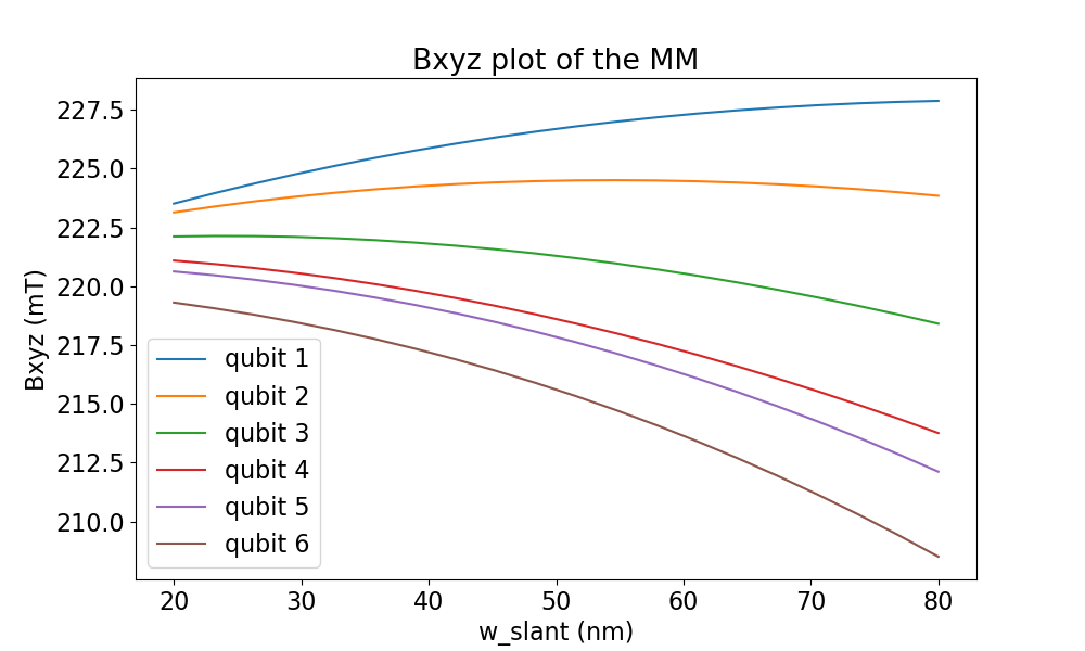
view.plot_fields('xyz')

view.unit = 'mT'
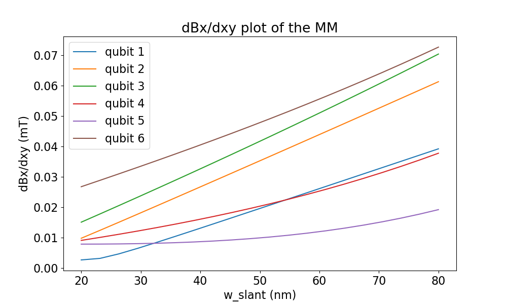
view.plot_derivative('x', movement_direction='xy')
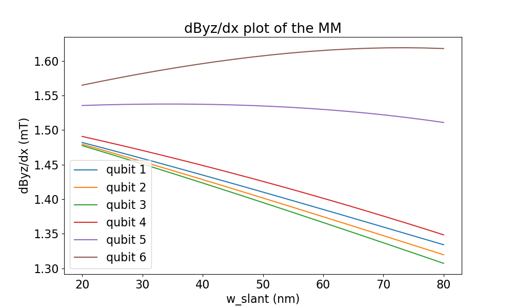
view.plot_derivative('yz', movement_direction='x')
view.show()

This code gives rise to the following plots :

Total field	Driving field	Decoherence field

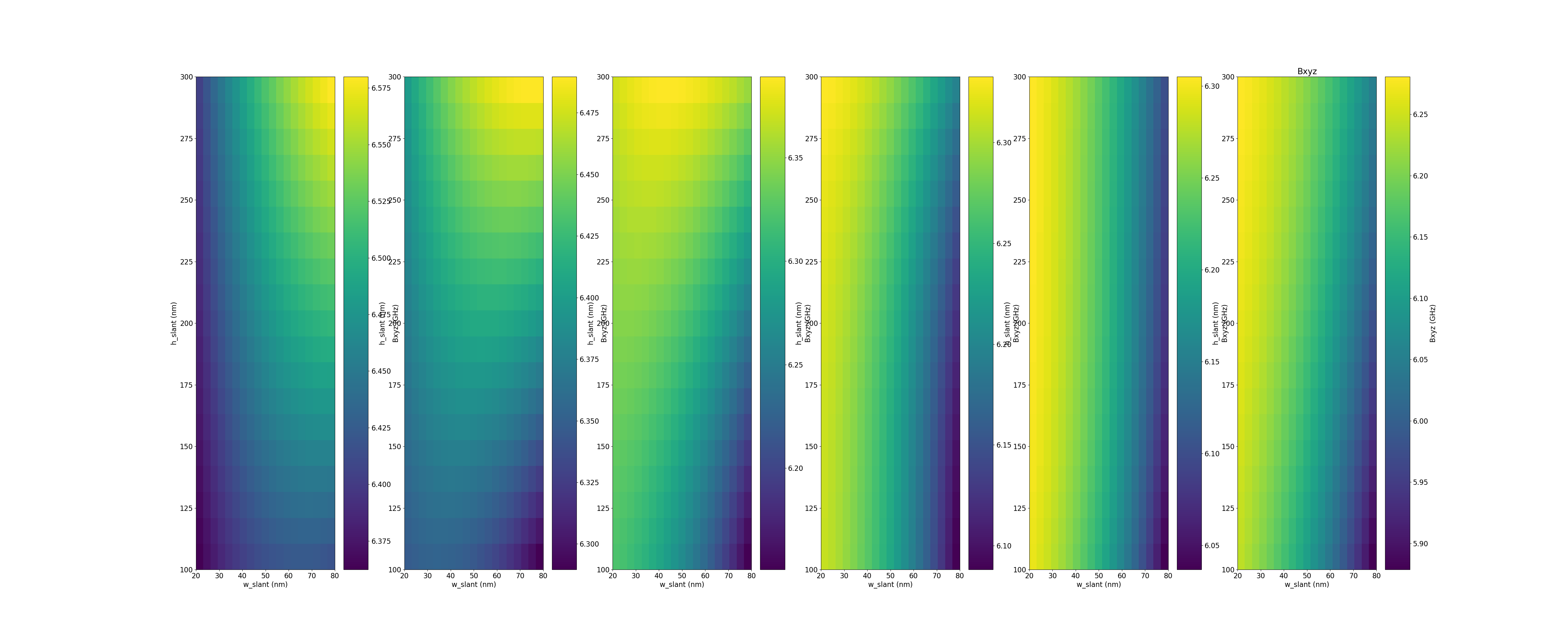
2D-sweeps

Example:

w_slant =  linspace(20, 80,20, axis=0, name='w_slant', unit='nm')
h_slant =  linspace(100, 300,20, axis=1, name='h_slant', unit='nm')

umag = example_MM_design(250, h_slant, w_slant)
view = umag.generate_qubit_prop()

view.unit = 'GHz'
view.plot_fields('xyz')

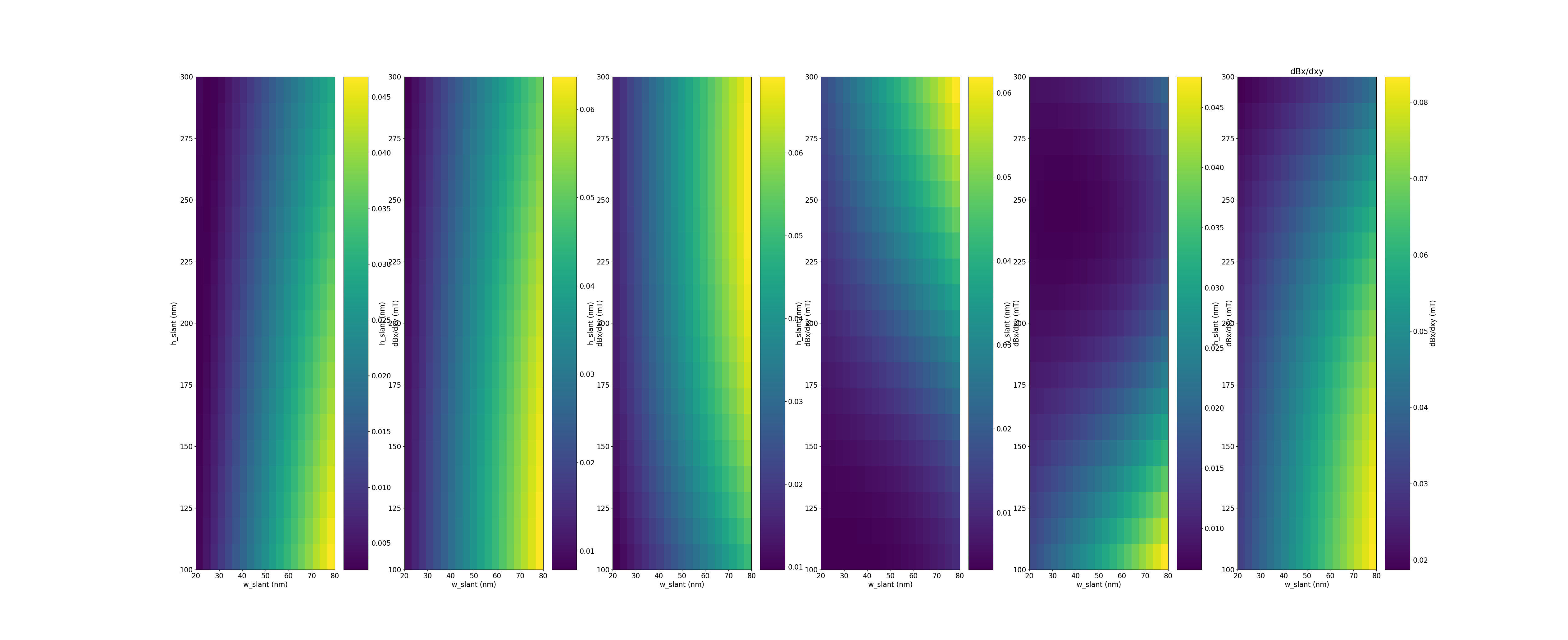
view.unit = 'mT'
view.plot_derivative('x', movement_direction='xy')
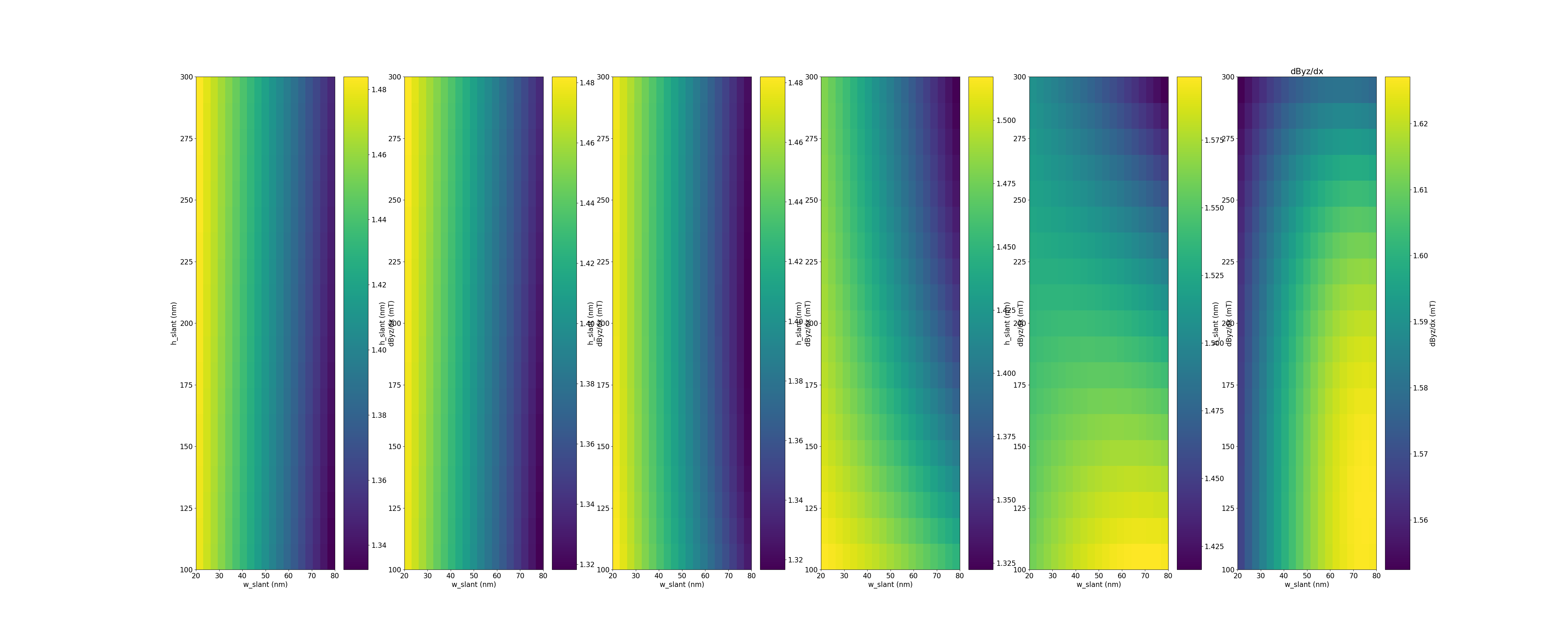
view.plot_derivative('yz', movement_direction='x')

view.show()

Results:

Total field	Driving field	Decoherence field